Simulating electrical activity in the small intestine
This blog post is the first article in what I hope will become a series dedicated to the simulation of physiological systems, with a focus on topic relevant to human anatomy and with at least some degree of clinical relevance.
A final disclaimer before we get started - I am not a health professional nor a professional researcher. I just enjoy learning about natural processes by attempting to model them - oh, and writing about that process as well. Inaccuracies and factual errors might slip in - feel free to reach out if you find some!
Model
Gastrointestinal motility refers to ability of the gastrointestinal tract to move contents across the system. This motility is driven by propagation of slow waves ([1]), which are generated by the interstitial cells of Cajal (ICC).
By studying electrical activity along the intestine, one can better understand the generation and propagation of those waves, as well as how the ICC layer interacts with the neighboring longitudinal muscle (LM) layer.
[2] introduces a non-linear model for electrical activity in the intestine. It is composed of the following partial differential equations:
v and i stand for the transmembrane potential and slow currents, respectively.
This model is derived from Van Der Pol oscillators, whose application to nerve modelling was first instigated by Richard Fitzhugh in [3]. The resulting Bonhoeffer-Van Der Pol model is then applied by Nagumo to model a nerve axon as an electrical transmission line in [4].
The model above is a modified version of equation 17 of [4], with the addition of coupling terms to model interactions between the ICC and the LM layers.
Implementation
We chose to use the Julia programming language to implement this model. Julia is a fast, dynamically typed language geared towards scientific computing. Official packages provide a lot of features, and the ecosystem also includes the excellent DifferentialEquations.jl [5] package, which we will use to solve the differential equations at hand. The full implementation is available here.
First, we need to define the two coupled intestinal layers of interest: the LM layer and the ICC layer. As mentioned above, the relevant parameters are discussed in the article:
struct LayerParams
    k::Float64
    a::Float64
    β::Float64
    γ::Float64
    ε::Float64
    D::Float64
    D_il::Float64
    α::Float64
end

const LM_PARAMS = LayerParams(
    10.0, 0.06, 0.0, 8.0, 0.15, 0.4, 0.3, 1.0
)

const ICC_PARAMS = LayerParams(
    7.0, 0.5, 0.5, 8.0, 0.15, 0.04, 0.3, -1.0
)
Then, we need to write two utility functions. The first one is an exponential decay, that we will use to compute the position-dependent
ε but also to compare the predicted intrinsic frequency of the ICC layer to our numerical results.
The coefficients used for ε were approximated from Fig. 2(b) found in [2], while the coefficients of the intrinsic
ICC frequency were extracted from [6]. The latter mentions an average 71 cm length content for the intrinsic
frequency for dogs, leading to a decay constant of 0.014.
function calculate_decay_parameter(x::Float64, total_length::Float64, start_val::Float64, end_val::Float64, decay_rate::Float64)
    r = x * total_length
    return end_val + (start_val - end_val) * exp(decay_rate * r)
end

calculate_epsilon(x, total_length) = calculate_decay_parameter(x, total_length, 0.0833, 0.03, -0.015)
calculate_intrinsic_frequency(x, total_length) = calculate_decay_parameter(x, total_length, 20.0, 10.25, -0.014)
Our model also features a laplacian to account for spatial coupling. We compute the laplacian exactly as described in [2], with the addition of a zero-flux boundary condition - which helps with numerical stability while preserving physical consistency - we assume that no electrical current flow in or out the extremities of the intestine.
function calculate_laplacian(u, idx, N)
    if idx == 1 # Julia arrays are 1-indexed
        return 2.0 * (u[idx+1] - u[idx])
    elseif idx == N
        return 2.0 * (u[idx-1] - u[idx])
    end
    return u[idx+1] + u[idx-1] - 2.0 * u[idx]
end
ODE solvers require users to formulate the explicit equation system - that system is then passed to the solver which will
handle stepping through the problem and attempt to converge towards a solution. Our formulation of the problem almost matches
the system of equations 1:1. Relevant quantities are packed in two vectors u and du. Note that we transform the PDE system
into a system of ordinary differential equations through discretization of the space and time dimensions.
function intestine_system!(du, u, p, t)
    N = NUM_CELLS
    v_lm  = @view u[1:N]
    i_lm  = @view u[N+1:2N]
    v_icc = @view u[2N+1:3N]
    i_icc = @view u[3N+1:4N]

    dv_lm  = @view du[1:N]
    di_lm  = @view du[N+1:2N]
    dv_icc = @view du[2N+1:3N]
    di_icc = @view du[3N+1:4N]

    for idx in 1:N
        x = (idx - 1) / (N - 1)  # Normalized position [0,1]

        # LM layer dynamics
        dv_lm[idx] = LM_PARAMS.k * v_lm[idx] * (v_lm[idx] - LM_PARAMS.a) * (1.0 - v_lm[idx]) -
                     i_lm[idx] +
                     LM_PARAMS.D * calculate_laplacian(v_lm, idx, N) +
                     LM_PARAMS.α * LM_PARAMS.D_il * (v_icc[idx] - v_lm[idx])
        di_lm[idx] = LM_PARAMS.ε * (LM_PARAMS.γ * (v_lm[idx] - LM_PARAMS.β) - i_lm[idx])

        # ICC layer dynamics (with position-dependent ε)
        local_ε = calculate_epsilon(x, TOTAL_LENGTH)
        dv_icc[idx] = ICC_PARAMS.k * v_icc[idx] * (v_icc[idx] - ICC_PARAMS.a) * (1.0 - v_icc[idx]) -
                      i_icc[idx] +
                      ICC_PARAMS.D * calculate_laplacian(v_icc, idx, N) +
                      ICC_PARAMS.α * ICC_PARAMS.D_il * (v_icc[idx] - v_lm[idx])
        di_icc[idx] = local_ε * (ICC_PARAMS.γ * (v_icc[idx] - ICC_PARAMS.β) - i_icc[idx])
    end
end
The only missing piece is then the simulation loop. It is worth noting that this is also were we set the initial excitation of the cellular system. For biological consistency, we set the initial conditions to a smooth pattern varying between 0 and 1 across the small intestine.
The Tsit5 solver is used with a small 1e-08 error tolerance and a maximum time step that matches the one used in the paper. That specific
solver is, according to the DifferentialEquations.jl docs,
a good algorithm for standard non-stiff problem (the non-stiffness of this problem is hinted at by the fact that the original authors were
able to solve it with a simple Euler method).
function simulate_intestine(tspan=(0.0, 75.0))
    u0 = zeros(4 * NUM_CELLS)

    # Apply initial stimulation with a phase gradient to both layers.
    stim_cells = 1:ceil(Int, NUM_CELLS)
    for i in stim_cells
        phase = 2π * (i - 1) / length(stim_cells)
        u0[i] = 0.5 * (1 + cos(phase))
        u0[2 * NUM_CELLS + i] = 0.5 * (1 + cos(phase))
    end

    prob = ODEProblem(intestine_system!, u0, tspan, ())
    sol = solve(prob, Tsit5(); abstol=1e-8, reltol=1e-8, dtmax=0.1)
    return sol
end
Results
We run the simulation using the same parameters as the reference article:
- 300 coupled cells (approx. 240 cm)
- Space step: 1
- Maximum time step: 0.05
The results presented in [2] hint at data capture being performed at a steady state. As such, we decide to run our simulation for 4000 seconds before starting to record data.
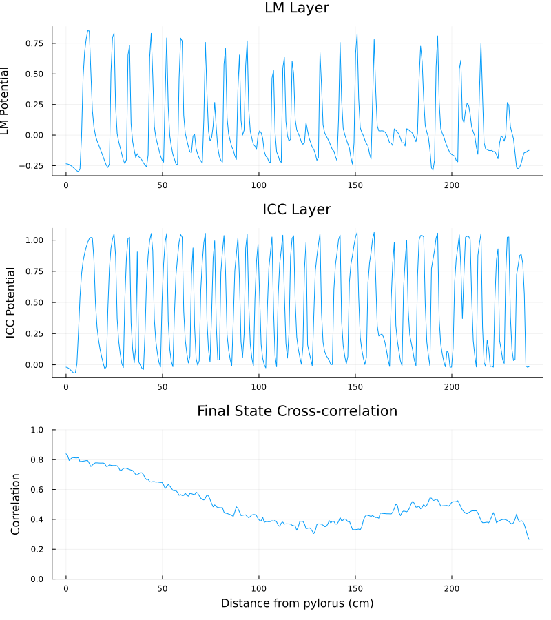
The figure below is a snapshot of the electrical waveforms across the LM and ICC layers for the spatial domain of interest. One can already notice that the cross-correlation between the two signals tends to be lower as one gets further from the pylorus (the part of the stomach that connects to the duodenum, which marks the start of the small intestine).
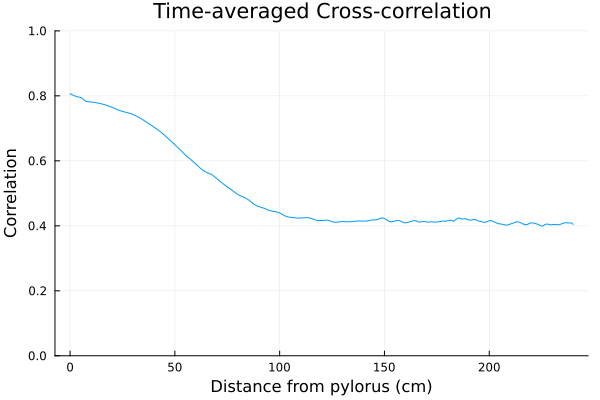
The cross-correlation profile between the two layers can be clearly identified by averaging cross-correlations over 1000 seconds.
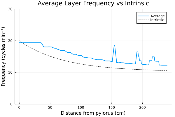
One of the key results of [2] is the ability of the model to simulate experimental observations (see [6]) - the figure below is obtained by averaging the frequency profile of the ICC and the LM layers along the spatial domain over 1000 seconds. The intrinsic curve represents experimental observations.
Our implementation reflects the figures presented in the reference article, with an initial threshold followed by exponential decay and chaotic oscillations towards the end of the domain. A discussion of those results can be found in [2].
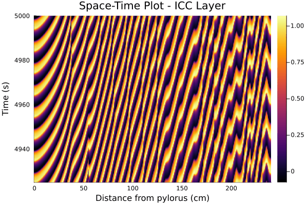
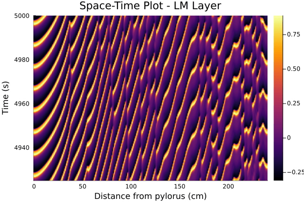
The two figures below have an equivalent in [2], and provide a clear visualisation of the transmembrane potentials getting desynchronized as they progress along the intestine.
